
What to look for when using forecasts from NWP models for streamflow forecasting?
There have been a few posts on NWP performance lately, and so we thought we’d add our perspective. We’ve been working closely with the Bureau of Meteorology to extend their new 7-day deterministic streamflow forecasting service to an operational ensemble streamflow forecasting service. One of the fundamental choices we have to make is the source of quantitative precipitation forecasts (QPFs). This is not as straightforward as it may seem – QPFs that show strong performance in some ways may not be suitable in others, while even if a hypothetical ‘ideal’ QPF exists, it may not be useable e.g. because it is inconsistent with other forecasts the Bureau issues.
Here’re some of the things we look for in QPFs from Numerical Weather Prediction (NWP) models:
- QPFs that perform best after post-processing. We use a post-processor to produce ensemble forecasts from deterministic QPFs (we call it the Rainfall Post-Processor or RPP; see Robertson et al., 2013). It’s a little similar to EMOS-type post-processors (see, e.g. Gneiting et. al; 2005) with which you may be familiar. Post-processors are able to correct many of the deficiencies of rainfall forecasts, so we are looking for QPFs that add extra information.
- QPFs that produce skilful forecasts in a range of catchments. The goal is to apply a single system across all of Australia, so we need to handle all the conditions Australia throws at us: from tropical/monsoonal climates, through arid areas, to cool temperate climates.
- QPFs that produce skilful forecasts of accumulated rainfalls. Yes, the timing of rain storms is very important, and we of course consider this when we evaluate QPFs. But for streamflow forecasting, the total amount of rainfall (irrespective of timing) forecasted for all lead-times can be crucial. Assessing the performance of accumulated rainfall forecasts – particularly for measures of reliability – is not commonly considered in literature published on evaluating QPFs.
In Australia, the Bureau of Meteorology uses the ACCESS suite of NWP models and the‘Poor Man’s Ensemble’ (PME) to provide guidance to issue official weather forecasts. The PME is simply a collection of 8 deterministic NWP models. The global version of ACCESS (ACCESS-G) is developed and operated by the Bureau to produce 10-day deterministic rainfall forecasts, while the PME form the major basis of operational weather forecasting products issued by the Bureau. The Bureau asked us to evaluate if ACCESS or PME would be preferable for an ensemble streamflow forecasting system.
After post-processing there is little to separate the performance of PME from ACCESS-G across a range of catchments (Figure 1) – even where there are big differences in the performance (particularly bias) of the raw forecasts, such as for tropical Queensland. As you can see CRPS is almost identical for raw ACCESS-G and PME, but the bias is vastly different. The PME has a tendency to predict too many small rain events because of “smearing out” rainfall from component models in the ensemble mean. These small positive errors help cancel out a few significant negative errors (underestimation) which leads to smaller bias in PME. In contrast, the small positive errors add up with the negative errors when computing CRPS (absolute error for deterministic forecast).

Figure 1. Catchment average rainfall and CRPS in the raw and calibrated rainfall forecasts in Tully (Queensland – Tropical) and North Esk (Tasmania – Temperate) catchments
Calibrated QPFs from ACCESS-G and PME are equally reliable at individual lead times (Figure 2). When we consider accumulated rainfall totals, the story becomes more interesting: reliability of calibrated PME QPFs is worse than calibrated ACCESS-G QPFs (thick lines in Figure 2). We suspect that this could be due to autocorrelation in raw PME forecasts. Taking the average of any set of deterministic forecasts will generally give a smoother (i.e., more autocorrelated) rainfall forecast than an individual NWP forecast. This autocorrelation isn’t compatible with the Schaake Shuffle (Clark et al., 2004), which we use to instil temporal and spatial correlations in the QPFs. (Though we’re not sure this is the cause – anyone else come across this problem?) Of course, the benefit of averaging many deterministic NWP models to produce the PME should be an increase in forecast accuracy – but in this case this advantage is only slight.

Figure 2. Probability Integral Transform – uniform probability diagrams (PIT plots) for the catchment average calibrated QPFs in Tully and North Esk catchments. Thin lines are for individual and thick lines – cumulative, yellow lines = calibrated ACCESS-G, violet lines – calibrated PME
Of course, in a brief blog post it’s not possible to cover all the aspects of NWP QPFs that interest us: for example, we are also very interested in the streamflow forecasts that are produced by our calibrated QPFs. So we’ll leave you to fill in the gaps:
- What makes a good QPF for you? What’s important to you when you assess QPFs for streamflow forecasts? Do you look for something others don’t?

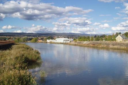
North Esk River in Launceston, Tasmania (Temperate/Perennial) (Creative Commons License)

Tully River in Far North Queensland (Tropical/Perennial) (Creative Commons License)

Ord River downstream of Lake Argyle in North East of Western Australia (Grassland/Intermittent) (permission from https://austravelphotography.files.wordpress.com)
Original article posted on HEPEX website, 26th July 2016 (Link)